Gippsland Basin Uncertainty Study
from IPython.core.display import HTML
css_file = 'pynoddy.css'
HTML(open(css_file, "r").read())
%matplotlib inline
#import the ususal libraries + the pynoddy UncertaintyAnalysis class

import sys, os, pynoddy
# from pynoddy.experiment.UncertaintyAnalysis import UncertaintyAnalysis

# adjust some settings for matplotlib
from matplotlib import rcParams
# print rcParams
rcParams['font.size'] = 15

# determine path of repository to set paths corretly below
repo_path = os.path.realpath('../..')
import pynoddy.history
import pynoddy.experiment.uncertainty_analysis
rcParams.update({'font.size': 20})
The Gippsland Basin Model
In this example we will apply the UncertaintyAnalysis class we have been
playing with in the previous example to a ‘realistic’ (though highly
simplified) geological model of the Gippsland Basin, a petroleum field
south of Victoria, Australia. The model has been included as part of the
PyNoddy directory, and can be found at
pynoddy/examples/GBasin_Ve1_V4.his
reload(pynoddy.history)
reload(pynoddy.output)
reload(pynoddy.experiment.uncertainty_analysis)
reload(pynoddy)

# the model itself is now part of the repository, in the examples directory:
history_file = os.path.join(repo_path, "examples/GBasin_Ve1_V4.his")
While we could hard-code parameter variations here, it is much easier to
store our statistical information in a csv file, so we load that
instead. This file accompanies the GBasin_Ve1_V4 model in the
pynoddy directory.
params = os.path.join(repo_path,"examples/gipps_params.csv")
Generate randomised model realisations
Now we have all the information required to perform a Monte-Carlo based uncertainty analysis. In this example we will generate 100 model realisations and use them to estimate the information entropy of each voxel in the model, and hence visualise uncertainty. It is worth noting that in reality we would need to produce several thousand model realisations in order to adequately sample the model space, however for convinience we only generate a small number of models here.
# %%timeit   # Uncomment to test execution time
ua = pynoddy.experiment.uncertainty_analysis.UncertaintyAnalysis(history_file, params)
ua.estimate_uncertainty(100,verbose=False)
A few utility functions for visualising uncertainty have been included
in the UncertaintyAnalysis class, and can be used to gain an
understanding of the most uncertain parts of the Gippsland Basin. The
probabability voxets for each lithology can also be accessed using
ua.p_block[lithology_id], and the information entropy voxset
accessed using ua.e_block.
Note that the Gippsland Basin model has been computed with a vertical exaggeration of 3, in order to highlight vertical structure.
ua.plot_section(direction='x',data=ua.block)
ua.plot_entropy(direction='x')
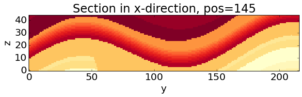
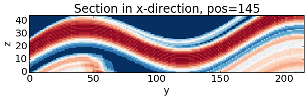
It is immediately apparent (and not particularly surprising) that uncertainty in the Gippsland Basin model is concentrated around the thin (but economically interesting) formations comprising the La Trobe and Strzelecki Groups. The faults in the model also contribute to this uncertainty, though not by a huge amount.
Exporting results to VTK for visualisation
It is also possible (and useful!) to export the uncertainty information to .vtk format for 3D analysis in software such as ParaView. This can be done as follows:
ua.extent_x = 29000
ua.extent_y = 21600
ua.extent_z = 4500

output_path = os.path.join(repo_path,"sandbox/GBasin_Uncertainty")
ua.export_to_vtk(vtk_filename=output_path,data=ua.e_block)
The resulting vtr file can (in the sandbox directory) can now be loaded and properly analysed in a 3D visualisation package such as ParaView.
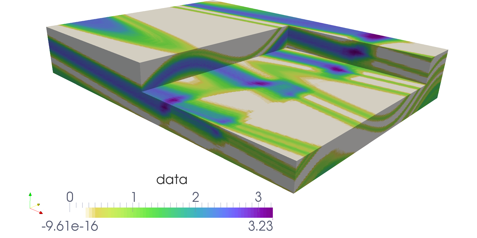
3-D visualisation of cell information entropy